1 Greater than the Sum of its Parts
Outline
Emergence
The brain is often described as the most complicated device in the known universe.[1] The basic units of information processing in the brain are neurons and glial cells. Yet, neurons and glial cells aren’t generally considered to be terribly intelligent on their own. At a certain level of description, on which you’ll read more later, neurons and glials cells could be thought of as dominoes, reacting simply to local conditions around them. Somehow, though, putting together 86 billion neurons and a similar number of glial cells—about 200 billion dominoes—produces something REALLY intelligent. How?
For more details on neurophysiology, see part II of the Open Educational Resource An Introduction to Neuroscience. For a shorter introduction, see Cells of the Nervous System.
To understand your brain is to understand the concept of emergence. Stephen Hawking, a brilliant modern physicist, has called the study of emergence the science of the 21st century.[2] Emergence is often described by the mantra “the whole is greater than the sum of the parts”.
Water is a canonical example of emergence. You could define water as H20, a molecule composed of two hydrogen atoms and one oxygen atom. However, this would be an incomplete description. To understand this, think about the following:
Think Critically 1.1
Liquidity is a property of the interaction of H2O molecules. Emergence is often found when you have many things (like H2O molecules) interacting. Let’s reflect on what is emerging here. Nothing about your knowledge of hydrogen or oxygen would allow you to predict the myriad of properties of water, including surface tension (which allows leaves and bugs to sit on the surface), a high capacity to hold heat (which buffers the earth from large temperature fluctuations, and is also why temperatures are more temperate near a large lake than further away), and the feeling of wetness. Most importantly, water provides a medium for molecules to dissolve, chemical reactions to occur, and materials to be transported—all properties which make water essential to life on earth. Clearly, the whole (water) is greater than the sum of the parts (hydrogen and oxygen atoms).
Two other illustrative examples of emergence are diamonds and graphite. Diamonds and graphite (which can be found on the end of a pencil) are chemically identical. Both are collections of interconnected carbon atoms. And yet they appear quite distinct: graphite is opaque, diamonds are transparent; graphite is soft, diamonds are hard. The key difference is how the carbon atoms interact—carbon atoms are arranged differently in diamonds and graphite, as shown below, and those different arrangements account for the diametrically opposed properties of the two substances!

For even more fascinating examples of emergence, watch this video:
Interactions amongst a large number of elements are the critical factor in emergence. Interacting H2O molecules give rise to properties much different than a single H2O molecule, or either hydrogen or oxygen atoms. Different interactions of carbon atoms give rise to radically different types of material. Likewise, the sophistication of the brain emerges out of the interactions of relatively simple neurons. Interactions are crucial for intelligence.
Because interactions are so critical, it is important to gain greater familiarity with the wonder of emergence, and the types of patterns and behaviors that can be generated by different types of interactions. Activity 1.1 is a straightforward example of emergence that a group of people can demonstrate. Before doing the demonstration, try to predict what the results would be!
Activity 1.1: Emergence of Walking Patterns
Gather a group of people (6 or more) in an enclosed space (for example, a classroom, or a demarcated space outside). Each person should choose a random starting location within the space. Each person then follows two rules:
- If no one is immediately in front of you, walk randomly. That is, turn whenever and in whichever direction you feel like.
- If there is a person immediately in front of you, simply follow them.
What patterns did you observe emerge? Did the pattern change over time? Try changing the group’s size—do different patterns emerge with increasing group size?
Activity 1.1 illustrates an important principle: even very simple rules of interaction can give rise to unexpected—and sometimes complex—patterns. The rules defined the nature of your interactions, which catalysed the emergent patterns.
Cellular Automata
Emergence can be systematically studied using a class of computer models called cellular automata. Computer models are important for studying emergent systems (like the brain) because the results of having a large number of interacting agents (like neurons) are often difficult to predict and hard, if not impossible, to work out by hand.
By way of introduction to cellular automata, imagine a square on a piece of graph paper (see Activity 1.2 below). That square can either be filled-in with a pencil, or left white. Which state the square is in (filled-in or blank) depends on the states of the square’s neighbours: simple rules link the state of a square to the state of that square’s neighbours. In a so-called “one-dimensional (1-D)” cellular automaton, the fate of a given square depends on just three neighbours: the square immediately above it, the square one up and one to the left, and the square one up and one to the right, as in the box in Activity 1.2 below (those three squares form a short line, which is 1-dimensional, hence the cellular automaton’s description as a 1-D cellular automaton). The figures in Activity 1.2 represent one possible rule set for linking the state of the bottom square to the states of its three top neighbours. Our rule set must indicate whether the bottom square should be filled-in black (“B”) or left white (“W”) for every possible combination of the states of the three squares above it. Since each of the top squares can be in two states, and there are three squares, there are 23 = 8 combinations of top squares. For each of the eight combinations, the rule set below shows what the bottom square should be (B or W). To see which pattern emerges from this rule set, do Activity 1.2.
Activity 1.2: 1-D Cellular Automaton
This activity requires either a piece of graph paper or a spreadsheet (e.g., Excel or Google Sheets). In whichever you are using, mark off a space consisting of 21 columns and 20 rows. In the center of the top row, fill in one square. That square is now black (B), while all the rest of the squares in that row are white (W). Now apply the rule shown in the figure below, in the following way:
- To begin, start with the left-most square of the second row. For this square, the square up and to the left does not exist (it is off outside of the boundary), so consider it as not filled in, or white (W). The square immediately above our target square is white (W), as is the square up and to the right. Looking below, we see that when the top row has squares that are W W W, the target square is W, which means it should be left unshaded (white).
- Now apply the same procedure to the next square to the right. There are three squares above, all of which are white (W). And so you would leave that square white as well.
- You can readily see that this pattern will repeat as you move the “target square”, the square you are trying to figure out if it should stay white (W) or be filled-in black (B), until you approach the central square you filled in at the start of this activity.
- For a particular target square, the three squares above it will be W W B, because the central square has been filled in. What should you do with the target square in this case, according to the rule below?
- When your target square becomes the next square to the right, the pattern above that square become W B W. What do you now?
- Continue moving to the right, determining whether to leave a square white or turn it black. When you reach the right-side of the page, assume that any missing squares are W.
- Now, move one row down and begin again at the left side. Continue moving left to right, applying the rule below until you finish the last row.
- When you are done, you can check you work by moving the slider in the image below to the right. This shows the results of this rule if you had been able to fill in many more rows and columns. You should recognize the top portion of the pattern mirrored in the one you created.
As you can see, a simple rule iterated repeatedly gave rise to quite an unexpected pattern. Indeed, the pattern you derived is known as a fractal. Fractals are patterns that repeat themselves at multiple scales. In the image that you generated, within the larger triangle were a few smaller triangles, within which were a few smaller triangles, etc. Trees are another classic example of a fractal: trees have a large trunk with branches coming off of it, each branch has a main trunk with branches coming off of it, etc. If you were looking at a close-up of a single branch without contextual clues, it would be unclear if you were looking at a small tree, or the smaller branch of a large tree. Your body is also composed of a lot of fractal structures. Blood vessels are fractals (using the same reasoning as for trees), your respiratory system is fractal, and dendrites (the receiving ends of neurons) are fractals. Fractals are important biologically because complete structures can be produced with simple rules. Your DNA generates complex structures like your cardiovascular, respiratory, and nervous systems by encoding the simple rules of production for those systems, rather than exactly what the end structure should look like. In other words, fractals give you a lot of bang for your genetic buck. This helps explain in part how it can be that humans have the same number of genes as the much smaller mouse!

For a very interesting introduction to fractals, watch the video below!
Activity 1.2 represents just one rule. We could have chosen the opposite state for each of the bottom squares. B could have been W and vice-versa. Because each of the eight combinations of the three top squares can map onto two possible states of the bottom square, there are 28 = 256 possible rule sets. In other words, there are 256 ways that four squares—which can only be blank or filled-in—can interact! The sheer number of possible patterns emerging from these rules dramatizes why computer models are important. Let’s turn to a computer model to see these other rule sets (do Activity 1.3).
Activity 1.3: 1-D Cellular Automata in Netlogo
- Download Netlogo,[3] which is a free modeling platform for examining emergence.
- In Netlogo, click File –> Models Library. Expand the Computer Science folder, and then expand the Cellular Automata folder. Open CA 1D Elementary.[4]
- Click on the Information panel and read its contents.
- Go back to the Interface panel, and click on “setup single”—this fills in one square in the middle of the top row, just as you did to start Activity 1.1.
- Under “Rule switches”, scroll to Rule 18 and hit “go”—this should produce the same pattern you created manually and saw as the solution to Activity 1.2 (though the colors of the foreground and background may be different).
- Now set rule to 1 and click on “setup single”. Quickly scroll though all 256 Rules to get a feel for the types and diversity of patterns produced. Each time you select a new rule, you must click “setup single”, then “go”.
- Feel free to play around with the other parameters and see what happens.
Now let’s get a little more concrete, and see an example cellular automaton which models a real world phenomenon. In the next Activity (1.4), you’ll see how cellular automata can reproduce different fur coloration patterns—from the striping of zebras to the spotting of Dalmatians. This cellular automaton is more complex than the last one—now the state of a cell is a function of the cells above it, below it, and to the sides. In other words, this is a two-dimensional cellular automaton.
Activity 1.4: Fur
- In Netlogo, open the “Fur”[5] program, located in the Biology folder.
- Click on the Information panel and read its contents.[6]
- Return to the Interface tab and run the model several times (hit setup, then go). What happens? Hit setup and go a few more times. Why are the striping patterns different each time you run the simulation?
- Run the model with different INITIAL-DENSITY settings. Notice how, if at all, the value of the INITIAL-DENSITY affects the emergent pattern.
- In one sense, striping is a very robust phenomenon because it appears to be insensitive to the initial density of pigmentation. Now, however, note how sensitive striping is to slight changes in other parameters. If you hold all other factors and slightly change just the RATIO, from trial to trial, you will note that for small ratios you will invariably get completely white fur and for high ratios you will invariably get completely black fur. Why?
- For ratios in between it fluctuates. Describe some of the different patterns that emerge.
- Reset Density to 50% and ratio to .35. Change the inner-radius-y to 2. Describe the differences you see compared to when the inner-radius-y was the same as inner-radius-x. Explain these differences.
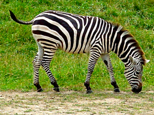
Note the striking qualitative similarity in the images below. The top image was generated using the Fur model in Netlogo. The middle image shows a similar striping pattern in a zebra’s coat. Finally, the bottom image depicts stains of “ocular dominance columns” in the primary visual cortex of a macaque monkey. The white stripes correspond to cortex with cells dedicated to processing visual input from one eye and the black stripes correspond to cortex with cells dedicated to processing visual input from the other eye. This qualitative similarity between images suggests similar dynamic interactions are at work in all three. What differs are the kinds of cells doing the interacting!


Both computers and brains are kinds of cellular automata.[7] Rather than B or W, imagine that the two possible states are 0 or 1. You have all probably heard that computers, at bottom, run on a series of 0s and 1s. What this means physically is that a particular electronic component either does or does not have electricity flowing through it. Whether or not electricity is flowing through a particular component is a function of whether or not electricity was flowing through some combination of its neighbors. Neurons can be thought of similarly. Whether a neuron is firing an action potential (1) or not (0) is a function of the activity of the neighboring neurons feeding into it. Just as 1-D and 2-D cellular automata generated unexpected and sophisticated patterns based on simple rules, so too are networks of neurons capable of unexpected and sophisticated processing, as you’ll see in the next chapter.
- Understanding emergence is central to understanding how the brain’s sophisticated information processing can arise from the relatively simple functioning of neurons.
- Emergence means “the whole is greater than the sum of its parts”.
- The properties of water and the differential properties of diamonds and graphite exemplify emergence.
- Emergence can occur when large numbers of elements interact with each other, often following fairly simple rules.
- Emergence may be systematically studied using a class of computer programs called cellular automata.
- One-dimensional (1-D) cellular automata demonstrate that simple rules can give rise to a diversity of unpredicted, and sometimes sophisticated patterns.
- Some 1-D cellular automata generate fractals: self-similar patterns at multiple scales. Fractals are also found in many natural and biological systems.
- Two-dimensional (2-D) cellular automata exhibit an even greater range of patterns.
- Some patterns are qualitatively similar to those found in biological systems—from the coloring of animal coats to the organization of the primary visual cortex in some animals, suggesting similar dynamic and operational principles.
- Both computers and brains can be thought of as cellular automata.
Media Attributions
- Diamond_and_graphite2 is licensed under a CC BY-SA (Attribution ShareAlike) license
- Tree_Fractal © Laurenjessiehatch is licensed under a CC BY-SA (Attribution ShareAlike) license
- CA Stripes © Christopher J. May
- Grazing_Zebra © Shonebrooks is licensed under a CC BY-SA (Attribution ShareAlike) license
- Ocular Dominance Columns © Valerie Hedges is licensed under a CC BY-NC-SA (Attribution NonCommercial ShareAlike) license
- If you read the Preface, you'll know that I've already complicated this claim, but it's still a useful rhetorical opening. 🙂 ↵
- Stephen Hawking said, “I think the next century will be the century of complexity” on January 23, 2000 in the San Jose Mercury News. Complexity is the study of emergence. ↵
- Wilensky, U. (1999). NetLogo. http://ccl.northwestern.edu/netlogo/. Center for Connected Learning and Computer-Based Modeling, Northwestern University, Evanston, IL. ↵
- Wilensky, U. (1998). NetLogo CA 1D Elementary model. http://ccl.northwestern.edu/netlogo/models/CA1DElementary. Center for Connected Learning and Computer-Based Modeling, Northwestern University, Evanston, IL ↵
- Wilensky, U. (2003). NetLogo Fur model. http://ccl.northwestern.edu/netlogo/models/Fur. Center for Connected Learning and Computer-Based Modeling, Northwestern University, Evanston, IL. ↵
- The explanation of w and the equation used to compute the pigmentation of a given cell is not clear. D*I and D*A don't mean D multiplied by I or A. They are just awkward variable names for the number of Inhibitors (D*I) or Activators (D*A). w is a weight. By multiplying w by D*I, you can adjust the strength of D*I. To reduce the influence of the inhibitors (D*I), you would reduce w. In the Interface tab, “w” is represented as “ratio”. The equation for computing the identity of a particular cell is: Identity = D*A - w(D*I). If Identity is > 0, the central cell is set to D (White). If Identity is < 0, the central cell is set to U (Black). If Identity is = 0, the central cell is unchanged. ↵
- Indeed, Stephen Wolfram, a pioneer in cellular automaton research, believes that the entire universe can be modeled as cellular automata. For more, see a TED talk from Stephen Wolfram. ↵
