We imagine that you may not be entirely satisfied with solely describing, however rigorously, the daily rhythm you’ve now demonstrated (see previous chapter).  Like other great discoveries, yours should also generate more questions than answers.  But the issue is:

What is your question?

There are numerous questions that could be tackled, for sure, but based on budgetary time and effort, available person-power, and your own lifespan, we recommend first choosing wisely and focusing on one of them to get your experiments underway.  In this chapter we put forward and discuss three broad questions; procedurally they are somewhat separate but conceptually quite interdependent.

***

Question 1: What are the mechanisms for generation & expression of daily rhythms?

This kind of question is of the type that seeks to understand how a biological process occurs (“proximate” causation), nowadays most often by employing reductionistic approaches.  We begin with the assumption that the parameters of the daily rhythm of interest – its period, phase, amplitude, and mean level – are shaped by multiple sources to form the final, composite, overt rhythmic waveform; generally speaking, some influences will arise externally outside the organism (exogenous), while other factors will be generated by the organism itself (endogenous).  Over a couple of hundred years, the existence of an internal timekeeping component – popularly known as the “circadian clock,” the subject of this book – was proven, and here we discuss three experimental strategies for revealing the presence and influence of circadian clocks through the dissection of daily rhythms into their exogenous and endogenous components.

a. Rhythm dissection in an environment without external time cues: 

Considerable effort has been expended in the laboratory to remove rhythmic external timing cues that might be driving daily biological rhythms or impacting their shapes, especially the alternation of light/darkness and high/low temperatures over 24 h (but including other conceivable cues as well) ^2.1.  Such direct effects on rhythm expression are referred to as “masking” – because they mask (hide) the presence or action of any endogenous timing element from the investigator’s view – and will be discussed in additional detail later in this chapter.  In any case, the experimental elimination of such masking effects leads to a stunning result: (a) the persistence of rhythmicity for many daily rhythms under such constant conditions, and (b) an expressed period that is relatively precise but with a value that may deviate considerably from 24 h ^2.2.  The period is thus circadian (“about a day” or “around a day”), referred to as “free-running” (that is, free of 24-h external synchronization), and its value denoted by the lower-case Greek letter tau (𝝉).

Under these conditions, the passage of internal biological time (“circadian time”) no longer matches that of local time, as defined by the light-dark cycle.  This situation calls for a special nomenclature (Fig. 5).

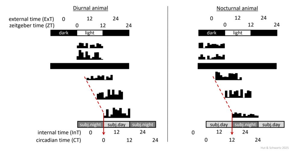
Actograms of a diurnally-active (left) and nocturnally-active (right) animal, initially maintained in a 12 h: 12 h light-dark cycle and then free-running in constant darkness.  Dotted red line indicates activity onset as a phase marker during constant darkness.
In the cases shown here, the value of 𝝉 is greater (longer) than 24 h; or, put another way, the rhythm is running slower than 24 h.

At least for a daily rhythm expressed in the presence of a light-dark (often abbreviated as LD) cycle, the simplest convention would seem to be the one that is already familiar to us: setting local time point “0” to the middle of the dark phase and partitioning the entire cycle into 24 equal hourly segments (this is akin to our concept of “midnight,” even though our local 12:00 AM does not always occur at mid-dark phase).  This solution has been designated “External Time” (ExT), with the number of hours elapsed since “0,” as in “lights-on at ExT 10 and off at ExT 22” (or other combinations that might not be 12 h of light and 12 h of dark).

You have undoubtedly encountered the term “zeitgeber” Time (ZT).  Zeitgeber is a German word (capitalized as a noun) for “timer” or “timegiver.”  Like ExT, ZT also denotes the passage of local time in the presence of a repeating 24-h timing cue, and is likewise divided into 24 equal hours, but ZT 0 is assigned as the time point of lights-on.  Traditionally, this scheme has been applied to the nomenclature of free-running rhythms in constant conditions, where “Circadian Time” 0 (CT 0) represents a projection over time of the previous ZT 0.  Using a single phase marker per circadian cycle allows partitioning the cycle into 24 equal parts, now as circadian hours, with one circadian hour = 𝝉/24 h (of note, for one circadian hour to have the same duration across all phases of the cycle, the speed (velocity) of the oscillation is considered to be constant across all phases of the cycle).  For a nocturnal animal like a mouse or hamster, the clear activity onset may serve as a convenient phase marker for each circadian cycle.  Since activity onset during a light-dark cycle occurs at the onset of darkness (ZT 12), activity onset under free-running conditions may serve as the phase marker for CT 12.  So, for a mouse with a circadian period length around 23.7 h in constant darkness, under these conditions one circadian hour = 23.7/24 = 0.9875 h.

The terms “subjective day” and “subjective night” are used to represent projections of the preceding light and dark phases, respectively, over circadian time; this definition is thus irrespective of the timing of an organism’s usual activity and rest phases (thus, CT 0 is identical for a diurnally active human and a nocturnally active mouse).  Of course, the ExT terminology can be analogously extended in constant conditions to “Internal Time” (InT).  A significant advantage of the ExT/InT over ZT/CT configuration becomes evident when comparing rhythms under different photoperiods (light phase durations); with the changing seasons in nature, both dawn and dusk shift to different relative phases of the cycle rather than one of them (dawn, ZT 0) remaining anchored and immovable by definition.

An actogram is a very effective graphical display for visualizing 𝝉 and for its visual estimation via an eye fit line through activity onsets (Fig. 6).

 

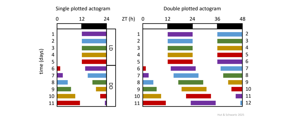
Stylized actograms of a nocturnally-active animal under a 12 h: 12 h light-dark cycle (LD) released into constant darkness (DD).  The double-plotted actogram repeats the format for 48 h, where day n is followed by day n + 1 horizontally, succeeded by day n + 1 and n + 2 on the next line, then by day n + 2 and n + 3, and so on.  The double plot design allows for the visualization of an unbroken free run.

In practice, most of the attention to constant conditions in the laboratory has focused on lighting, and the classical procedure has been to employ constant darkness (DD).  Although the use of constant light (LL) was key to the early discovery and analysis of circadian rhythms in plants ^2.3, its effects tend to be complicated, especially for animals that exhibit rhythmic sleep-wake cycles with the eyes alternately closed and open ^2.4.  In studies of humans in temporal isolation, whose behavior can be directed, a “constant routine” protocol seeks to unmask the innermost kernel of the circadian timekeeping machinery underlying physiological rhythms, especially for the body temperature rhythm.  In addition to the elimination of external light and temperature cycles, the protocol also minimizes willful rest-activity patterns such as physical activity and posture, intermittent meal timing, and sleep.  In this way, estimation of the relative contribution of the “central” internal timekeeper to the ultimate, integrated waveform of the overt natural rhythm might be feasible.  A similar approach has been attempted to dissect other daily physiological rhythms, such as blood pressure.  Constant routine protocols are understandably short in duration given the intensive monitoring involved.  Moreover, a significant confound of the protocol is an associated and inevitable element of sleep deprivation, and perhaps also the continued presence of ambient dim light.

In 1979, a very simple linear diagram of an archetypical circadian system was published, inspired by work on the experimental dissection of daily rhythms, now commonly referred to as the “Eskinogram” (Fig. 7) ^2.5 .

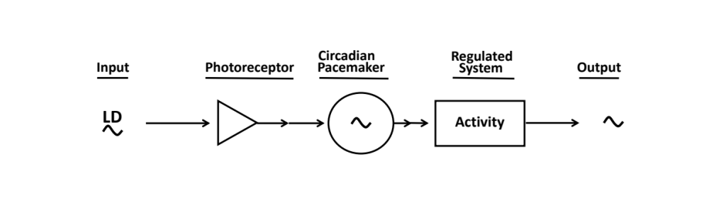
Drawn from: Eskin A. Identification and physiology of circadian pacemakers. Fed Proc 38:2570-2572, 1979.

A critical feature of the model is the non-identity of the central timekeeper (“circadian pacemaker”) from the observable rhythm that it either drives, regulates, or generates (“output” via a separate “regulated system”).  This sequential segregation means that an output rhythm can be eliminated or altered somehow downstream of the pacemaker – become dissociated from it – without interrupting or affecting the continued timekeeping by the pacemaker itself ^2.6.  An “output” rhythm is not necessarily a faithful, passive “read out” of the state of the upstream pacemaker, as might be implicit in the diagram.  As we have discussed above, the “regulated system” must be integrating the circadian signal along with a number of non-circadian ones to mold an output rhythm with phase, amplitude, and waveform that might not replicate the pacemaker’s parameters.  Furthermore, and importantly, how we as investigators choose to assay output rhythms may alter properties and performance of the system itself.  For example, locomotor activity in fruit flies and rodents can be measured using a variety of apparatuses, most popularly with Drosophila activity monitoring (DAM) systems and rodent running wheels, respectively, but our methods may have an impact on features of circadian timekeeping per se ^2.7.  In humans, one of the attractive features of using the nocturnal rhythm of pineal melatonin levels to monitor circadian timing is its relative stability and tight regulation in the face of physiological, pharmacological, and behavioral variables (although production of the hormone is suppressed by bright light).

By the way, we tend to habitually and casually refer to “the free running circadian period” as though it were a fixed value for an individual, strain, or species.  However, it is a dynamic value, influenced not only by the running wheel but also by the intensity of constant light ^2.8, preceding lighting conditions (so-called after-effects), age, sex, and other factors.  The statistical approaches traditionally employed in biological rhythm research require that the data are stationary over time (that is, of unchanging period, amplitude, and waveform from the 1^st to the n^th cycle).  For rhythms that are non-stationary, a different analytical toolkit applies ^2.9.

b. Rhythm dissection by genetic and/or physical lesions:

In a sense, this strategy is the opposite of the one that removes exogenous timing cues.  Instead, here the aim is to modify or remove suspected endogenous timing elements, seeking telltale changes in the free-running period or even frank arrhythmicity (in the circadian range) as evidence that an endogenous timer has been impacted.

As is well documented, thanks to this strategy and to the power of molecular genetics and neurobiology, our knowledge of circadian systems made spectacular progress in the latter part of the 20^th century.  A genetic substrate underlying circadian rhythmicity had already been surmised in the 1930’s in studies of plant hybrids and populations of fruit flies maintained in constant light over multiple generations.  In the early 1970’s, mutations at single genetic loci in Neurospora (frequency [frq]) and Drosophila (period [per]) were generated that led to abnormally fast, slow, or absent rhythms; and by the 1990’s, a framework for the architecture of the core oscillatory machinery emerged, based on intracellular transcriptional-translational negative feedback loop(s) with built-in adjustable time delays ^2.10.  Meanwhile, in the 1960’s, destructive lesions of multiple brain areas and organs in rats focused specific attention on a critical role for the hypothalamus in generating circadian locomotor activity rhythms.  By the 1980’s, the suprachiasmatic nucleus (SCN) had been shown to exhibit properties expected of the central circadian pacemaker envisioned in the Eskinogram; and at the end of that decade came the impressive rescue of arrhythmic SCN-lesioned hamsters by fetal SCN transplants, with the values of 𝝉 (of wheel-running activity) restored in the hosts dependent on donor genotype ^2.11.  Continued work using these and increasingly sophisticated techniques has elegantly mapped circadian systems at the molecular, cellular, tissue, and whole organismal levels of biological organization.

It is customary to assess the phenotypes of lesioned organisms and preparations under constant conditions, because in some cases rhythmicity can appear normal if a recurrent 24-h exogenous time cue is present (that is, masking; for example, locomotor activity in a light-dark cycle).  There are other confounds inherent in genetic and physical lesion-making that are well known.  Identical mutations on different genetic backgrounds may have dramatically different phenotypic effects ^2.12, and there are remarkable examples of organisms’ capacity for functionally compensating for lost parts, especially but not exclusively during development ^2.13.  For this reason, it is prudent to keep in mind that some lesion phenotypes might actually reflect more about how an organism successfully (or unsuccessfully) adapts to the loss of specific genetic and anatomical elements than about how these elements function under normal conditions.  Also interesting to consider are cases labeled as “no phenotype,” since latent vulnerabilities of such systems might be concealed under favorable laboratory environments, only to be revealed by challenges such as sickness, stress, aging, or natural conditions.

A plethora of abnormal metabolic, physiological, and behavioral phenotypes has been associated with circadian arrhythmicity following the experimental elimination of some essential “clock” genes (for example, bmal1), raising exciting hypotheses about the possible roles of circadian dysfunction in the etiology, pathogenesis, and symptomatology of disease.  Here it is key to remember that “clock” gene activity is pleiotropic and not restricted to the core transcriptional-translational timing loop; bmal1, for instance, encodes a multifunctional transcription factor that regulates expression of a large portion of the genome (see Summary).  Thus, inactivation of the core circadian timing loop by knocking out a critical “clock” gene might also lead to a state of persistently high or persistently low expression of many circadian-controlled, downstream transcripts.  Resulting pathological mechanisms, or even the presence or absence of pathology per se, may therefore depend on how circadian arrhythmicity is being induced, whether by interruption of the positive or the negative limbs of the molecular oscillator’s feedback loop ^2.14.

c. Rhythm dissection by “forced desynchronization”:

In humans, the “forced desynchrony” strategy is a non-invasive behavioral manipulation that aims to disentangle rhythms of physical activity, meals, and sleep from the core circadian timing signal.  However, rather than eliminating these behavioral rhythms through a “constant routine,” forced desynchrony schedules participants to follow relatively normal daily routines but with sleep opportunities and meal times cycling with abnormally short or long periods of 20 or 28 hours, usually in a dim, very low amplitude light-dark regimen.  Circadian body temperature and melatonin rhythms cannot synchronize to these extreme periods (see limits of entrainment, discussed in Question 2 of this chapter) and instead oscillate with a period believed to approximate 𝝉 (Fig. 8).  Thus, over the course of this imposed desynchrony, as the dissociated behavioral and circadian rhythms cycle past each other, a series of changing phase relationships is generated between them; typically, these protocols should be continued long enough for all possible phase combinations to be expressed (a “beat cycle”).  Then by averaging the data over either the circadian or sleep/wake time axes, the relative contributions of behavioral and circadian rhythms on each other’s profiles can be estimated.

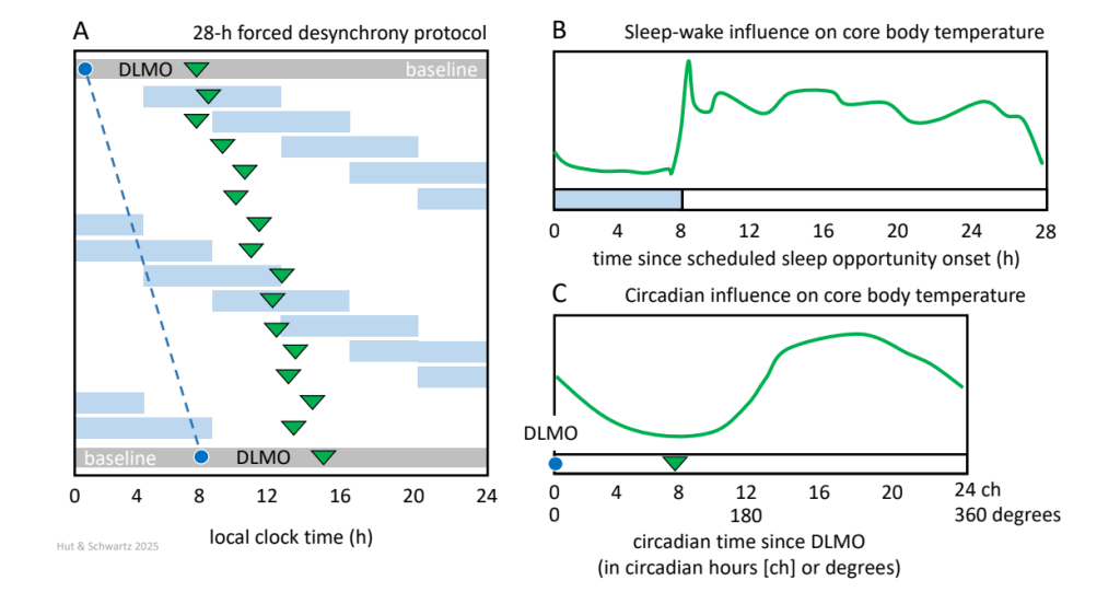
Shown is a stylized forced desynchrony (FD) protocol with a scheduled sleep-wake cycle of 28 h with an 8-h scheduled sleep opportunity (A; blue bars).  The protocol begins after an initial baseline day in which dim light melatonin onset is measured (DLMO, dark blue dot). DLMO is measured again after the FD protocol.  The 28-h FD protocol lasts for two beat cycles, meaning that the 12 sleep-wake cycles cover two times all phases of a full daily cycle (12×28 h=14×24 h=336 h) and approximately two times all phases of the yet to be established circadian cycle.  The period of the circadian cycle can be estimated post-hoc using the final DLMO measurement after the FD schedule.  In this example, initial DLMO=02:00 h, final DLMO=09:30 h, thus free-running period = 24 h + (7.5 h over 15 d)=24.5 h (indicated by the dashed dark blue line). Core body temperature is measured continuously, and for each circadian cycle the timing of core body temperature minimum is indicated (green triangles), which reveals the nature of its free-running circadian regulation.  Measurements like body temperature obtained during the protocol can now be binned and plotted on a sleep-wake-related time scale (in hours after sleep onset; B) and on a circadian time scale (in hours after interpolated DLMO; C).

This method has been especially useful in humans ^2.15  for assessing, for example, intrinsic circadian periodicity as well as the complex regulation of wakefulness, sleep efficiency, sleep stages, and other variables.  Thus, the rhythm of wakefulness is seen to be impacted by both circadian- and sleep-dependent processes: it is lowest (and sleep latency the shortest) around the minimum of the body temperature rhythm, while wakefulness within sleep episodes increases as a function of elapsed time within the episode.  An additional finding is that the circadian contribution to the regulation of rapid eye movement and slow-wave (delta) sleep stages differs significantly, with an influence on the former considerably greater than the latter.  Notably, an inherent feature of the forced desynchrony protocol – that is, the varying alignments expressed between central circadian (presumably SCN) cycles and behavioral (fasting/feeding and sleep/wake) cycles over time – reveals that such temporal disruption can result in physiological and metabolic consequences that are likely to be clinically relevant.

***

Question 2: What is the functional utility of a circadian clock?

This kind of question is of the type that seeks to better understand the evolution of a biological process and how it contributes to enhanced adaptation to the environment (fitness), eventually leading to increased lifetime reproduction (“ultimate” causation).  Raising this question about the adaptive functions of a system can in turn guide the focus of investigations at the proximate level.

It is of course a truism that most all organisms on earth are faced with a host of 24-h cycling stimuli, presenting both challenges and opportunities for synchronization.  We use the term synchronization here in its most restrictive sense, courtesy of the Oxford English Dictionary, as “coincidence or agreement in point of time;” that is, simultaneity, as in synchronized swimming.  It is certainly possible for organisms to synchronize some of their functions and behaviors to the day or to the night without the need of a circadian clock.  One such synchronizing mechanism is the phenomenon we referred to as “masking” in Question 1 of this chapter, as may be observed in animals with genetic and/or physical lesions of their circadian pacemakers that express apparently normal locomotor activity rhythms when they are maintained in the presence of a light-dark cycle.  Importantly, a clock-less state is not a necessary condition for masking; recall our discussion of the human “constant routine” protocol, in which certain behavioral patterns are suppressed with the aim to “unmask” the innermost circadian timing signal underlying the body temperature rhythm.

Although a sound physiological mechanism, masking is ultimately a reactive one ^2.16.  Without an internal sense of time, there is no possibility for anticipating a recurring external event (for example, morning lights-on or periodic food availability) and preparing for it ^2.17.  Such an internal sense allows not only for anticipation but also for the dynamic regulation of optimal rhythm phases – synchronizing compatible processes, separating incompatible ones, properly sequencing others, and tuning temporal organization in response to environmental circumstances.  An adaptable timekeeping mechanism should be favored by evolution and key to an organism’s selective advantage in nature.  Indeed, in the relatively few species that have been studied both in nature and the laboratory, the phases and waveforms of some daily rhythms are plastic and can differ dramatically between the two conditions ^2.18.  Across biological kingdoms, the ubiquity of internal timekeeping systems that enable such adaptable phase control is a testament to the benefits of a clock mechanism that essentially represents the external day-night cycle within organisms rather than having them simply react to it.  Such a mechanism not only ensures the organism’s external alignment to daily environment cycles but also the internal alignment of its metabolic, physiological, and behavioral rhythms to each other.

Obviously, this function demands that the circadian oscillator adopts a stable phase relationship to the day-night cycle.  Entrainment is the process by which two oscillating systems assume the same period – in our case, 24 h – generally with one driving (entraining) the other, thereby establishing a stable phase relationship between them over succeeding cycles.  Their entrained phases may be synchronous (that is, with a “phase difference” or “phase angle difference” of 0°) or not (for example, in antiphase, at 180°).  Note that in our case, with the entrainment of two qualitatively different oscillating systems (rhythms of living matter to the day-night cycle), we can define the phase of entrainment between them as we wish by our choice of a phase reference point (e.g., onset, offset, peak, or center of gravity of rhythmic behavioral activity).  Obviously, the reference point(s) become a practically important decision for real-world rhythms that may not be sinusoidal or symmetrical.

a. Circadian entrainment by the light-dark cycle and discrete light pulses:

Theoretically, there must be a multitude of candidate entrainment cues (referred to collectively as Zeitgebers), but the most prominent ones (and the most intensively studied) are light and temperature, alone or in combination ^2.19. The role of a Zeitgeber in circadian entrainment can be demonstrated using a “jet lag” protocol, especially popular in laboratory studies of nocturnal rodents (although, admittedly, jet lag is not a condition represented in their evolutionary history).  By the way, to our knowledge, this experimental approach was first reported and presented in actogram format in 1926 ^2.20, well before there were jet airplanes or jet lag.

We have found that the descriptive vocabulary of jet lag can be confusing for students or newcomers to the field, so let us begin with the actual problem that most of us may have experienced (Fig. 9).  Imagine a non-stop flight from Boston’s Logan Airport (BOS) to Amsterdam’s Schiphol Airport (AMS) (Fig. 9A); they are 6 time zones apart, with local AMS time ahead – later than – local BOS time (since the Earth rotates from west to east, the sun rises at AMS 6 hours earlier than at BOS).  Now, with a favorable tailwind, flight duration from BOS to AMS will be about 6 hours.  A BOS departure at 19:00 local time + 6 hours in flight results in an AMS arrival at 01:00 the next day from the traveler’s perspective, whose subjective (internal) time is still set to local BOS time.  Of course, the problem is that local AMS time is actually 07:00, so re-entrainment to the new local time requires that our traveler’s rhythm must advance or speed up towards it; another way of expressing this is that external AMS phase reference points – say, the morning (lights-on) or a dinner reservation – will now come earlier than expected from a BOS point of view.  The same logic can be applied to the return trip from AMS to BOS (Fig. 9B), with local BOS time behind – earlier than – local AMS time.  Now on this leg there is likely a headwind, so flight duration from AMS to BOS will be about 8 hours.  An AMS departure at 12:00 local time + 8 hours in flight results in a BOS arrival at 20:00 the same day from the traveler’s perspective, whose internal time is still set to local AMS time.  Of course, the problem is that local BOS time is actually 14:00, so re-entrainment to the new local time requires that our traveler’s rhythm must delay or slow down towards it; another way of expressing this is that an external BOS phase reference point – say, the dinner reservation or bedtime (lights-off) – will now come later than expected from an AMS point of view.  Note that in this example the BOS to AMS traveler flies in the direction of the Earth’s rotation while the AMS to BOS traveler flies against it; at these roughly realistic departure times, the former compresses the duration of their night, while the latter expands the duration of their day.

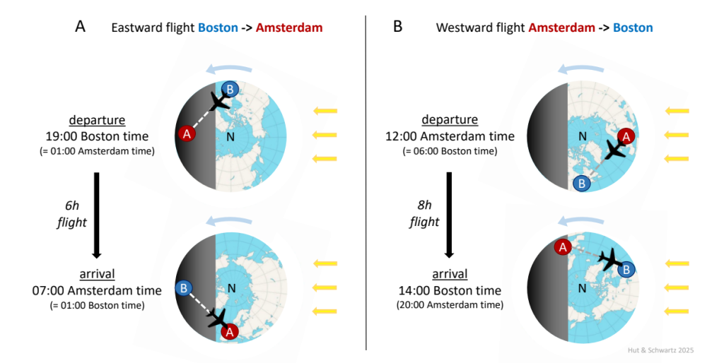
Polar views of the Earth (N, north pole) rotating from west to east (blue arrow) with the sun illuminating daytime in the northern hemisphere during summer (yellow arrows).  Local time in Amsterdam (red circle A) is 6 hours ahead (later than) local time in Boston (blue circle B).

In the typical laboratory experiment (Fig. 10), the animal (usually a mouse, hamster, or rat) is initially maintained on a 24-h light-dark cycle (on the order of weeks, generally as a 12 h: 12 h light-dark schedule) and locomotor activity monitored (by running wheel or infrared beam sensor); ordinarily, daily activity onset will occur around lights-off.  Then, the timing of the light-dark cycle is abruptly shifted; for example, with lights-on and lights-off now occurring 6 h earlier the next day (Fig. 10A).  Over several days, animal activity onset gradually advances each 24-h cycle until it is re-aligned with the new lights-off.  The shifted light-dark cycle has re-entrained the circadian pacemaker that drives the locomotor activity rhythm, and the process is referred to as a phase advance of the pacemaker (or the rhythm).  The opposite re-entrainment maneuver – with lights-on and lights-off occurring 6 h later the next day (Fig. 10B) – is referred to as a phase delay.

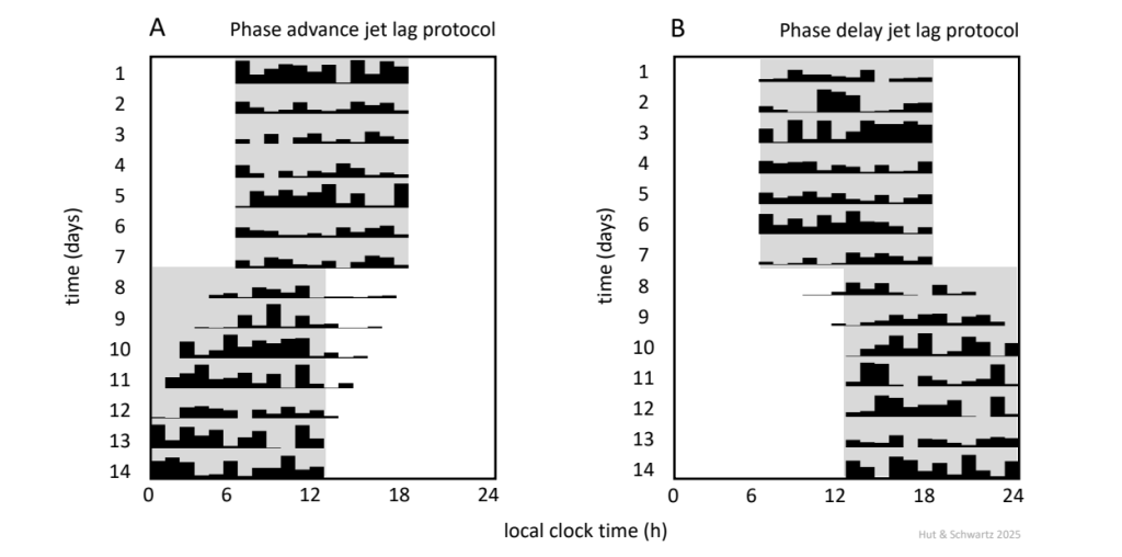
Actograms of two nocturnally-active animals, initially maintained in a 12 h: 12 h light-dark cycle and then subjected to a 6-h advance (A) or delay (B) of the cycle.  Shading represents darkness.  Note the difference between the advance and delay shifts in the speed of re-alignment of activity onset.

But wait!  Is synchronization after the shift in the light-dark cycle due to entrainment of the circadian pacemaker or to “masking” of the locomotor activity rhythm?  The answer in the illustrated case depends on the marker being used to track rhythm phase and the direction of the induced shift.  If the marker is activity onset – as it often is, since onset is usually easily and reproducibly identified in nocturnal rodents – its slow movement over several days (referred to as transients) during the phase advance (Fig. 10A) argues for entrainment as a mechanism.  On the other hand, activity onset during the phase delay appears to shift immediately and completely (Fig. 10B).  This asymmetry in the speed of re-entrainment hints at a possible role for masking in the delay direction, because the shifted light phase in that direction is initially coincident with the animal’s activity phase (and the masking effect of light is known to suppress the expression of locomotor activity in nocturnal rodents).  In the ideal design to distinguish entrainment from masking, the jet lag protocol should be preceded and followed by measurement of the animal’s free-running rhythm in constant darkness.  If entrainment has occurred, the phase of activity onset after jet lag should clearly differ from that predicted by extrapolation of the pre-protocol free run (Fig. 11).

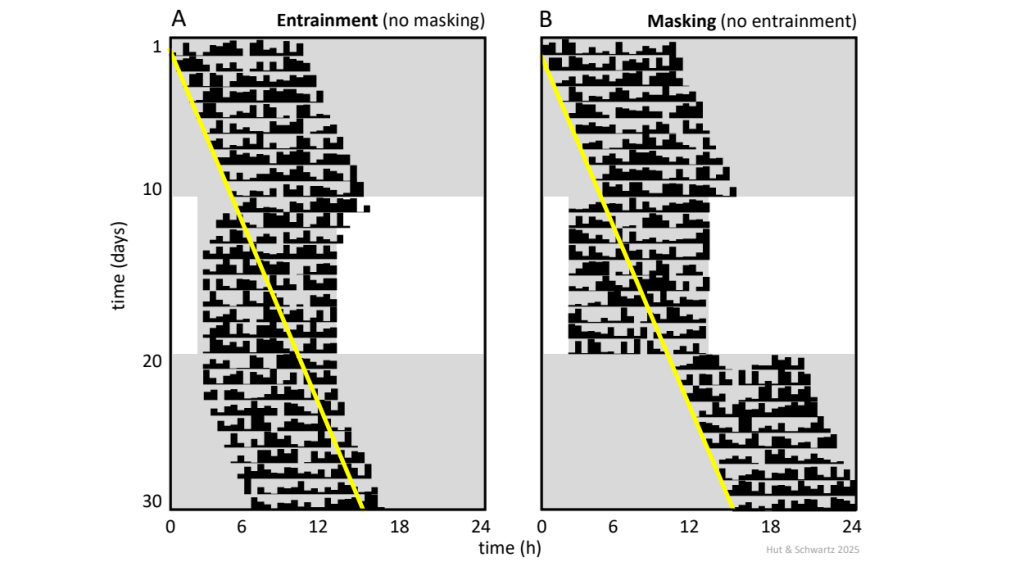
Shown is the “classical” experimental protocol to determine if synchronization of an activity rhythm to a light-dark cycle represents entrainment or masking (in this case, to a 12 h: 12 h light-dark cycle during days 11 – 20).  Shading represents darkness.  The key is to record free-running period in constant conditions before and after the synchronization interval.  With entrainment (A), the phase of the rhythm after synchronization (in this case, activity onset on day 21) is predicted by its phase just before release from synchronization.  With masking (B), the phase is instead predicted by extrapolation of the pre-protocol free run (yellow line), indicating that the underlying oscillator has continued to run unperturbed through the experiment, with synchronization of the activity rhythm due to a direct action of the light-dark cycle.  Note that the argument assumes an invariant value for the free-running period through the entire procedure.  Also shown in the figure are two additional characteristic features of entrainment: synchronization achieved gradually over several cycles (in this case, with 4 days of advancing “transients”) and the presence of an after-effect that reflects the preceding entrained period (in this case, the 2 initial days in constant darkness that express a period equal to 24 h).  Neither of these features is seen with masking.

The light-dark cycles we have been discussing can be described as complete photoperiods (in the case of Fig. 10, it is the 12 h duration of the light phase), and it is “complete” in the sense that light is continuous for the full 12 h interval.  Notably, stable entrainment and re-entrainment with jet lag can also be achieved under certain skeleton photoperiods, characterized by two short, discrete light pulses (say, 15 min to 1 h in length) that define the onset and offset of the light phase.  Interestingly, the differential speed of re-entrainment in the jet lag protocol – with delays completed quickly but advances only slowly after a series of transients – is also a feature of the protocol under a skeleton photoperiod, so differential masking cannot be the only explanation for the asymmetry in the shifts ^2.21.

Entrainment by discrete light pulses indicates that the circadian pacemaker shifts differentially to light applied at different phases across the circadian cycle, and a graph of such shifts as a function of the phase of light pulse administration can be plotted as a “phase response curve” (PRC) (Fig. 12).  The general configuration of the PRC is similar for all organisms, whether their behavior is diurnal, nocturnal, or something else; it is thus a property of the pacemaker itself.  Light pulses administered during the late subjective day / early subjective night (that is, around subjective lights-off [CT 12]) result in a phase delay (the pacemaker and rhythm move to a later phase); light pulses administered during the late subjective night / early subjective day (that is, around subjective lights-on [CT 0]) result in a phase advance (the pacemaker and rhythm move to an earlier phase); and light pulses administered during most of the subjective day have little effect.

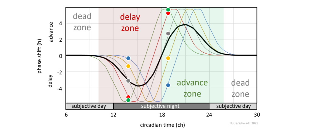
The canonical PRC to brief light pulses (black waveform), with delay phase shifts after light administered during the late subjective day / early subjective night, advance phase shifts during the late subjective night / early subjective day, and little or no phase shifts during most of the subjective day.  In practice, PRCs are experimentally derived from populations of animals, likely with inter-individual variation in their phases (see Fig. 3); here we show how such variation in individual data points from 5 animals might appear after light pulses around circadian times 13 – 14 and 19.  Note that the blue animal would actually exhibit a phase delay after a light pulse administered during the early part of the average “advance zone.”

The shape of the PRC suggests a provisional blueprint for natural entrainment of the circadian pacemaker to 24 h by daily phase shifts to light around dawn and dusk.  If the pacemaker’s period is too long – oscillating slower than once every 24 h – exposure to daily morning light will advance its phase; if the period is too short – oscillating faster than once every 24 h – exposure to daily evening light will delay its phase.  Quantitatively, with entrainment, the light induces phase shifts that exactly compensate for the period mismatch between the light-dark cycle and the free running pacemaker (Fig. 13).  In this way, the shape of the PRC and the difference between 𝝉 and 24 h determine a rhythm phase that is stable upon entrainment to the light-dark cycle.

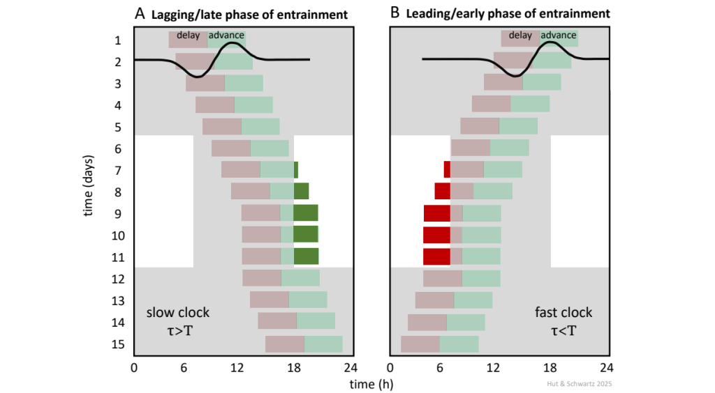
The free-running rhythms shown here represent the PRCs of two circadian oscillators with periods either longer (A) or shorter (B) than 24 h.  Shading represents darkness; advance (green) and delay (red) zones of the PRCs are as denoted in Fig. 12.  Both oscillators can be stably entrained to the 12 h: 12 h light-dark cycle but do so assuming different phases of entrainment.  When the circadian period is too long, exposure to daily morning light will advance oscillator phase; when the period is too short, exposure to daily evening light will delay oscillator phase.  Entrainment on day 9 occurs when the magnitude of the light-induced phase shift compensates for the difference between the periods of the free-running oscillator and the entraining cycle, expressed as 𝝉 – T =  Δφ, where 𝝉 is the circadian period, T is the entraining period, and Δφ is the magnitude of the phase shift.

The discrete (non-parametric) model of entrainment outlined above demonstrates considerable explanatory power and has been widely adopted.  And yet, it assumes that phase shifts are instantaneous, complete photoperiods are irrelevant, and 𝝉 is fixed (even though we know that the value of 𝝉 is altered by light; refer to ^2.8  on the shortening or lengthening of 𝝉 under constant light conditions).  So an alternative – the continuous (parametric) model – posits that light decelerates (slows down) or accelerates (speeds up) the pacemaker’s oscillation in a phase-dependent fashion, based on a velocity response curve qualitatively comparable to light’s non-parametric effects in constant darkness.  This model may help to resolve the conundrum of photic entrainment in animals that do not see dawn or dusk ^2.22.  Most likely, the truth involves aspects of both entrainment models.

b. 𝝉, light sensitivity, and phase of entrainment:

Regulating the phase of entrainment in nature – for example, as an “early bird” or a “night owl” – is surely critical for adapting to dynamic environmental challenges; so, from an evolutionary point of view, entrained phase would seem to be the pre-eminent circadian parameter undergoing natural selection ^2.23.  Mathematical analyses and simulations as well as experimental data have suggested that organisms could adjust their phase of entrainment to a 24-h Zeitgeber by regulating the pacemaker ‘s velocity (that is, the value of 𝝉) and/or its sensitivity to the entraining signal.

Experimentally, we don’t yet have a reliable method for systematically varying and clamping the pacemaker’s velocity in any one individual living organism.  However, we can vary the mismatch between 𝝉 and the entraining cycle (referred to as T) either by exploiting a range of short and long period mutants or by altering T across a range of non-24 h periods (T cycles) ^2.24. The results suggest that entrainment phase is a monotonic function of the degree of 𝝉 – T mismatch, as well as defining the range (limits) of entrainment to the shortest and longest T cycles, beyond which synchronization is not possible (recall the “forced desynchrony” protocol introduced earlier in this chapter).  Particular examples using golden hamsters show that these 𝝉 and T cycle influences on the phase of entrainment can be quite dramatic even in mammals ^2.25.

With regard to the role of the pacemaker’s sensitivity to the entraining signal, light is of course the most widespread and powerful 24-h Zeitgeber, and in the last decades spectacular progress has been made in our understanding of the photic entrainment pathway to the SCN.  These include its strictly ocular localization; the key role of the photopigment melanopsin (OPN4) expressed by multiple classes of intrinsically photosensitive retinal ganglion cells interacting with rods and cones; the responsible neurotransmitters, receptors, and second-messenger signal transduction pathways in the SCN itself; and ultimately in immediate-early and per gene transcription ^2.26.  Nevertheless, it remains experimentally difficult to systematically vary the photic sensitivity of circadian systems (as examples, altered sensitivity due to retinal adaptation or pupillary size), so the empirical approach has primarily focused on varying stimulus strength (irradiance, duration, and wavelength).  Increasing the photic “dose” will change the shape of the PRC, augmenting delays and/or advances by a few hours (a “type 1 PRC”, as in Fig. 12), and, in humans, increasing the degree of suppression of the nocturnal level of melatonin (light exposure via the SCN inhibits pineal melatonin synthesis and release; this suppression is thus used as a proxy to measure light sensitivity ^2.27).  In “lower” organisms (like fungi, insects) as well as some rodent genetic mutants, very large phase shifts around 12 h can be generated – so large that it may be impossible to classify them as advances or delays (a “type 0 PRC”) ^2.28.  As a practical matter, most routine laboratory experiments employ saturating light intensities (a couple of hundred lux for rodents) that may not be standardized across laboratories; “lux” is a measure based on human, not rodent, perception of brightness, and equal illuminance in lux is often not equivalent in the distribution of wavelengths and their intensities.  Importantly, measures of light exposure that account for species differences in wavelength sensitivities have been proposed recently ^2.29.

So the bottom line, generally speaking, is that phase of entrainment can be related to the magnitude of the 𝝉 – T mismatch and degree of Zeitgeber strength.  As a common rule: if 𝝉 < 24 h, and the greater the mismatch or the less the Zeitgeber strength, then the earlier the entrainment phase; if 𝝉 > 24 h, then the later the entrainment phase ^2.30.  But it is fair to say that quantitative prediction of the phase of any one individual remains a work in progress.  Modeling suggests additional oscillator properties need to be included – properties that may not be easily or unambiguously obtained in the laboratory – such as oscillator amplitude (the effective strength of the Zeitgeber is related to oscillator amplitude, increasing as amplitude decreases) and relaxation rate (for systems that switch between states, as with feedback loops of activators and repressors).  Additionally, and perhaps most inconveniently for simple models, populations of coupled oscillators – not only in the SCN and the Drosophila head but throughout the body (see Question 3 in this chapter) – can behave quite differently from the autonomous behavior of one oscillator alone ^2.31.  And ultimately, we must confront the complexity of entrainment in the natural world: where variance of light irradiance and spectral composition at actual dawn and dusk is not mimicked by our usual laboratory “lights-on” and “lights-off;” where 𝝉 is not a fixed unchanging value; where an array of non-photic biotic stimuli (with non-photic PRCs) appear irregularly; where age and sex are factors; and where “noise” in the photic entrainment signal is unavoidable.

***

Question 3: What is the systems physiology of circadian networks?

The cloning of circadian clock genes made possible the development of transgenic luciferase reporters of real-time circadian gene expression – and the subsequent discovery that the core molecular circadian timing loop oscillates in cells, tissues, and organs throughout the body (Fig. 14) (although already in the late 1950’s and early 60’s there had been claims that isolated rodent organs could express circadian rhythms) ^2.32.  We have since learned that cell-autonomous circadian rhythmicity is a ubiquitous feature of nearly all living matter – not only in certain bacteria, unicellular eukaryotes, and cell cultures & cell lines, but also nearly everywhere in multicellular organisms: in the cells of tissues, organs, brain regions, and cancers; endocrine, hematopoietic, and immune systems; and embodied parasites and symbionts.

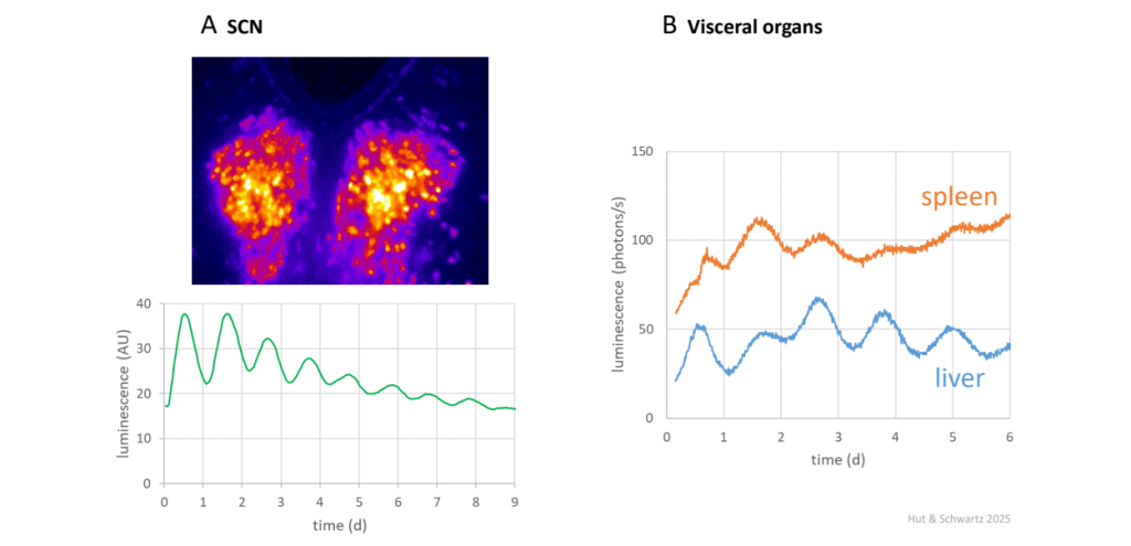
SCN (A) and visceral organs (B, spleen and liver) were obtained from mPer2^Luc knockin mice (Jackson Laboratory, Bar Harbor, Maine)  expressing a mPER2::LUC fusion protein; the mice were previously entrained to a 12 h: 12 h light-dark cycle.  The culture medium in the sealed culture dish includes the substrate luciferin, which emits light when metabolized by luciferase in the tissues, allowing real-time quantitative reporting of the amount of fusion protein.  Upper panel in (A), 9-day video recording of ~8.5 circadian cycles of the transgenic SCN ex vivo.

So now we find ourselves beyond the simple linear Eskinogram; deciphering the design principles of the timing of bodily functions will require a deep understanding of the dynamics of complex oscillator networks, coupled both within and across biological levels (from molecules to metabolic, physiological, and behavioral systems) and between anatomical regions.  For sure, this is a very hard problem!

a.  Conceptualizing the temporal architecture of circadian timekeeping:

The current conception of mammalian circadian organization is usually described as hierarchical. Typically, the SCN appears alone at the top, as the repository of the internal representation of the ambient light-dark cycle. External time (or circadian time, in constant conditions) is conveyed by the SCN to the brain and body via a panoply of neural, humoral, thermal, and behavioral signals ^2.33 that drive, gate, or entrain ^2.34 daily or circadian rhythmicity in downstream targets. In a cell-, tissue-, and organ-specific manner, combinations of these signals in concert with cellular energetic status engage the intracellular circadian timing loop to regulate circadian rhythms of gene expression. This regulation is mediated by mechanisms at different levels – including epigenetic regulation, transcription, RNA splicing, mRNA stability and translation, and post-translational modification ^2.35– ultimately leading to the flexible timing of biological functions. Customarily, the connectivity in this schema has been portrayed with multiple arrows projecting out from the SCN to its targets. The special position of the SCN at the pinnacle of the hierarchy is justified not only for its role in photic entrainment but also for its strong intercellular coupling – conferring precision and robustness to its output rhythms as well as resistance to the actions of its own downstream signaling modes (like feeding-, glucocorticoid-, and temperature-induced changes in phase) ^2.36.  Of note, temperature entrainment should not be confused with temperature compensation; the latter refers to a requisite property of a free-running rhythm with its period relatively resistant to differences in ambient temperature ^2.37.

A schematic diagram like the popular one described above is important for advancing scientific concepts because it helps to shape our mental models and the design of our experiments. So any re-working with additional data should reflect conceptual advances and not merely artistic refinements, and we do have some suggestions.  First of all, the exclusive position of the SCN as the pre-eminent circadian pacemaker in mammals is not conserved across other vertebrate classes; in some fish, reptiles, and birds, that function lies along an axis that includes not only an SCN but circadian pacemakers that are directly photoentrainable in retina and pineal gland ^2.38.  And second, that the isolated SCN continues to oscillate ex vivo does not mean that its cells are unresponsive to bodily influences in vivo. Indeed, the amplitude of its electrophysiological rhythm is altered by locomotor activity, and the nucleus receives many mono- and poly-synaptic neural afferents, bears receptors for molecules expressing rhythms that it controls, and responds to systemic cytokines ^2.39.  We need to learn much more about the SCN’s fine anatomy and compartmental organization, but these examples argue for a revised schematic that also includes a host of arrows projecting backwards, into the nucleus from the brain and body (Fig. 15).  It is tempting to imagine that the SCN and its extensive web of efferent signaling pathways has been co-opted by evolution to also meet unexpected homeostatic challenges to the internal milieu – such as starvation, dehydration, stress, inflammation, and activity state – that demand highly integrated metabolic, physiological, and behavioral responses ^2.40.

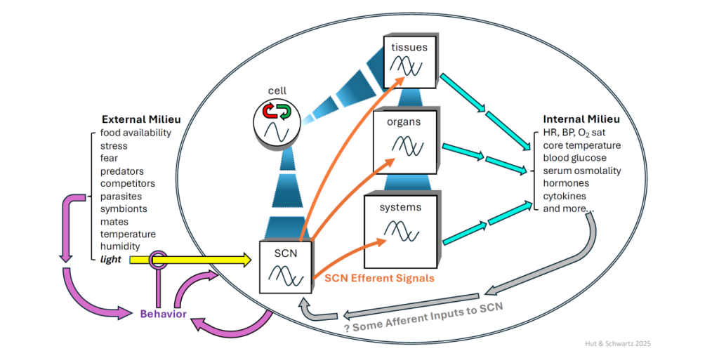
Within an organism (the oval bordered by a compound double line), the underlying oscillatory mechanism is within the cell, and cells form tissues, tissues build organs, and organs function together as physiological and metabolic systems.  In this schematic, the SCN is a specialized neural tissue embedded within the network.  On one hand, photic entrainment of its oscillation (yellow arrow) provides time-of-day information to tissues, organs, and systems via a variety of SCN efferent signaling mechanisms (orange arrows); on the other hand, the state of the internal milieu (green arrows) also appears to influence aspects of SCN rhythmicity (gray arrows), perhaps by modulating its electrophysiological activity and thus leading to possible consequences in efferent signaling.  Also shown are additional rhythmic features of the external milieu, some of which act through changes in behavior of the organism itself (purple arrows); and these altered  behaviors, in turn, may affect photic entrainment and masking.  Not included here are signaling mechanisms between organs (see ^2.41) nor tissue- and organ-specific Zeitgebers independent of the SCN (for example, local photic entrainment pathways [see ^2.42]).  HR, heart rate; BP, blood pressure; O₂ sat, oxygen saturation.

b. Phase alignment, realignment, and misalignment:

Sophisticated experimental techniques have been employed – including transgenic reporters for real-time tracking of rhythmicity in cells and tissues, optogenetics and chemogenetics, transcriptome profiling, and organ-specific conditional mutants – to discern how the architecture and dynamic connectivity of the circadian network leads to homeostasis at the level of the whole organism. The emerging picture appears extraordinarily complex.  Circadian gene expression in cells, tissues, and organs is not only determined by systemic signals and behaviors set by the SCN but also by the autonomous oscillators within the cells, tissues, and organs themselves; the resulting phase map is complicated by the fact that these local oscillators are not uniformly beholden to the SCN.  For metabolically active organs, the behavioral feeding-fasting cycle is a dominant Zeitgeber and remains so even when the behavior is uncoupled from SCN control (for example, by artificially displacing and restricting feeding to the light phase in a nocturnal animal); for skeletal muscle and lung, scheduled exercise has an analogous effect.  A host of candidate metabolites, hormones, neurotransmitters, and paracrine factors acting via specific receptor and second-messenger signal pathways underlies communication and coordination of rhythms and/or their local oscillators ^2.41.  Some of these oscillators – including in retina, cornea, and exposed skin in mammals – appear to be independently photoentrainable via activation of the photopigment neuropsin (OPN5) ^2.42.

It is through the proper alignment of rhythmic network components – for example, liver, pancreas, skeletal muscle, adipose tissue, intestine – that regulated blood glucose levels can be achieved even in the face of strong rhythms of feeding and fasting.  Crucially, alignments are malleable and adaptive; they are neither fixed internally within the network nor externally to geophysical time ^2.43.  The mechanisms underlying these kinds of readjustments of entrainment phase are not fully known, but from our discussion in this chapter (see Question 2, above), we can guess that such control might be mediated, at least in part, by changes in downstream oscillator 𝝉 and/or in the strength of oscillator coupling to resetting signals. The principles for how cell, tissue, and organ oscillators integrate multiple incoming signals, both in their quantity and quality, are not understood.

Establishing the daily temporal organization of biological systems requires coordination among multiple time axes: not only between external day-night (solar) time and internal body (circadian) time, but also behavioral (sleep) time and social or societal (clock) time, which in humans undergoes a yearly 1-h scheduled phase advance in spring and phase delay in autumn ^2.44.  Now given our appreciation of the complexity of the circadian timekeeping network, and the significance of optimal (and adaptable) alignment of its oscillating parts, a practical problem regarding circadian time becomes the definition and assessment of its phase with respect to the other axes, especially over repeated cycles in living animals. To this end, several measures have been promoted as indicators of mammalian phase of entrainment to the solar cycle. “Chronotype” is a word coined in 1974 to mean “temporal phenotype,” originally envisioned as a 24-h landscape of the distribution of peak phases of an array of rhythms in behavior, physiology, hormonal and biochemical levels, mitosis, circulating white blood cells, pharmacological sensitivities, and more ^2.45.  Since then, the term has been re-purposed as sleep phase, yielding practical insights on the variation of sleep timing relative to solar, circadian, or clock times, depending on lighting, age, sex, genetics, and even east-west position within a time zone. There are clinical consequences for individuals with extreme sleep phases, especially those that are delayed relative to modern societal school and work hours (Fig. 16).

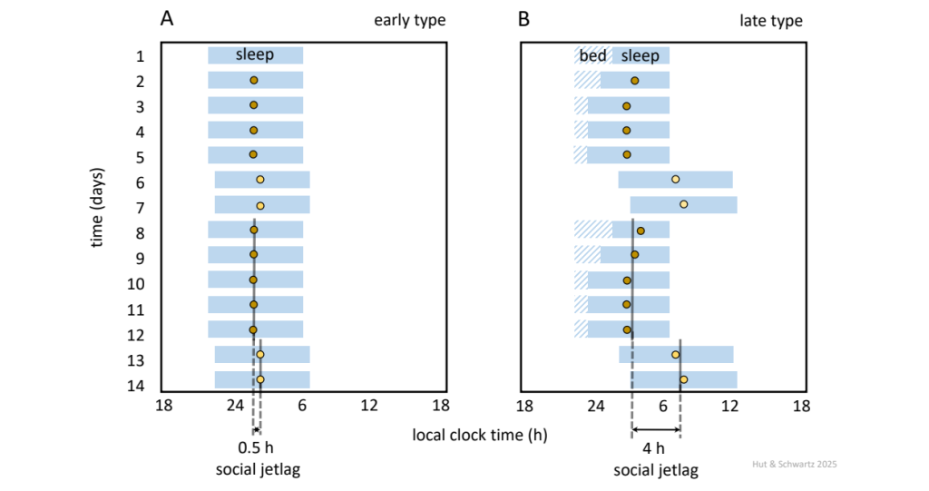
Stylized actograms of sleep duration and timing (blue bars) of two exemplary human chronotypes, early (A) and late (B), over 2 weeks of recording, with days 6/7 and 13/14 representing “free days” (weekends) unencumbered by alarm clocks or other social or societal demands.  Here, with both individuals required to awaken at 06:00 on “work days” (weekdays), the late type’s attempts to initiate sleep earlier than their natural late phase leads to sleep-onset insomnia (“bed,” hatched bars) and a shortened sleep duration.  This sleep deprivation during weekdays is compounded by “social jet lag” during weekends, when innately later sleep onset and wake up times generate phase delays and advances on Friday and Sunday evenings, respectively.  Measured as the difference in mid-sleep phase between weekdays and weekends (colored dots), the degree of social jet lag has been associated with cognitive, somatic, metabolic, and behavioral pathologies.

We have previously referred to the nocturnal rhythm of pineal melatonin synthesis and secretion as a reliable assay of circadian time, or at least as a gauge of “central SCN” time, with its phase in humans usually measured as rhythm onset under dim lighting conditions (dim light melatonin onset, or DLMO).  The rhythm is driven by the SCN via a well-described polysynaptic neural pathway, and, like the SCN, its phase is similar in diurnally- and nocturnally-active animals (for melatonin, high during nighttime in the dark, so phylogenetically it is a “darkness” hormone rather than a “sleep” hormone).  The key regulatory step in melatonin synthesis is in the activity of the enzyme aryl alkylamine N-acetyltransferase (AANAT); interestingly, the mechanism involves changes in AANAT gene transcription in rodents but not in ungulates or primates, reminding us that natural selection selects for outcomes, not necessarily for mechanisms.  On a discouraging practical note, however, most inbred laboratory mouse strains do not synthesize melatonin (including popular ones like C57BL/6 and BALB/c, but not including CBA and C3H), and even in humans multiple blood samples and specified lighting conditions are required to calculate DLMO.  Recently, there has been exciting work on developing novel assays of circadian time that may supplant DLMO, using one or two single blood samples for metabolomics or gene expression profiles of circulating blood cells ^2.46.

Equally exciting has been the increasing interest – among investigators and the lay public alike – in the causes and consequences of improper alignment of the circadian network to the time axes, as recognized in jet lag and shift work, and by several terms (disruption, desynchrony, misalignment) that attempt to acknowledge the myriad circumstances that could lead to circadian trouble.  These include, as examples, desynchrony due to differing periods between rhythms; misalignment due to anomalous phase relationships between rhythms; internal disruption within or between network levels; and external disruption between the network and the environment.  Such conditions have been associated with symptoms and signs of disease and health outcomes ^2.47, but interpretation of many of these associations will be a daunting task.  Which misalignments are adaptive (a physiological compensation to a challenge), which are pathogenic, and which are consequential rather than causal?  Which maladies result from associated disturbances of sleep rather than circadian misalignment per se?  Which misalignments are actually due to natural variation?  And what about the known confounds of most pre-clinical studies: laboratory mice, unlike most humans, are inbred, nocturnal, and as small rodents expend much of their energy defending body temperature.  On this point, typical animal facility temperatures lie below the lower critical temperature that defines the murine thermoneutral zone, so the alignment of the circadian network in our key model species during such “baseline” conditions actually represents a configuration under a metabolically stressful environment for them.

c.  Elaborating the clinical physiology of disturbed circadian function:

Our field has now developed the conceptual framework, investigative tools, and powerful analytics to further our understanding of the pathophysiology of circadian dysrhythmias. As the circadian system becomes a therapeutic target for pharmacological and behavioral interventions, humans are obviously the favored model, not only for their clinical relevance but also for the long tradition of applying holistic, integrative approaches to their study (including the recording of multiple rhythms from individual subjects).  We have emphasized from the beginning of this chapter that the expressed patterns of most daily rhythms are shaped by both endogenous and exogenous factors beyond the timing of clock genes. So now an important task will be work directed to understanding natural rhythm waveforms, aiming to estimate the relative contributions and weights of circadian and non-circadian influences.

Consider the case of body temperature, with (a) a value adaptively regulated (“tuned”) for optimal physiological performance via changes in heat production and/or heat loss, and (b) a rhythm, at least one function of which is acting as an internal 24-h Zeitgeber for the entrainment of some cellular and organ rhythms.  In adult humans, parameters of the overt temperature rhythm (mean level, range of oscillation, phase, waveform) can be altered by multiple factors, including ambient temperature, physical activity, sleep, meals, age, and the menstrual cycle.  Clearly, discovery of a disturbed temperature rhythm as part of a pathological state will require comprehensive studies to determine mechanistic connections and the arrow of causality, given the bidirectional relationship between circadian disruption and disease.

The daily rhythm of sleep and wakefulness provides another case study of an overt rhythm shaped by circadian and non-circadian influences.  Two key oscillatory processes, conceptually distinct but physiologically interconnected, interact to shape the nominal 8 h: 16 h waveform of the human sleep-wake rhythm.  One is circadian, based on internal time; the other relates to elapsed time, with the likelihood of sleep (known as sleep propensity or sleep pressure) increasing as a function of time spent awake and dissipating as a function of time spent asleep ^2.48 (a homeostatic regulation of sleep).  Forced desynchrony and other protocols have suggested how the combination of circadian and homeostatic influences might act to create the human consolidated but malleable sleep-wake rhythm (Fig. 17).

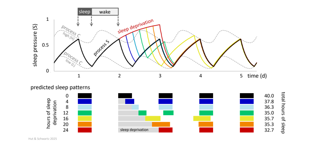
The two-process model was developed to account for the circadian influence on the timing of sleep and the response to sleep deprivation.  During wakefulness, sleep pressure (homeostatic process S, black curve) builds up by an inverse exponential increase that approaches an asymptote at 1; then during sleep, the pressure dissipates by an exponential decrease that approaches an asymptote at 0.  The switch from wakefulness to sleep, and from sleep to wakefulness, occurs when S reaches high and low threshold levels, respectively.  These levels fluctuate over 24 h following a skewed sines wave (circadian process C, high [H] and low [L] gray dashed curves).  The model (see references in ^2.48) has been instrumental, among other insights, in predicting the duration of sleep after prolonged deprivation (4 h, blue; 8 h, turquoise; 12 h, green; 16 h, yellow; 20 h, orange; 24 h, red), explaining the counterintuitive finding that sleep duration after 4 – 16 h of sleep deprivation is generally shorter than normal.

Note that an alternative schematic (Edgar, 1996; Dijk and Edgar, 1999) has focused on a circadian “alerting signal” that opposes a rising “sleep load” over the day, resulting in relatively stable wakefulness until the circadian signal declines in the evening.  Both models may not be very different, since the value of S – H might be a good measure of fatigue, and therefore H – S could be interpreted as an indicator of the circadian alerting signal.  

Edgar DM. Circadian control of sleep/wakefulness: Implications in shiftwork and therapeutic strategies. In: Physiological Basis of Occupational Health: Stressful Environments (Shiraki K, Sagawa S, Yousef MK, eds), Academic Publishing, Amsterdam, 1996, 1996, pp. 253-265.

Dijk DJ, Edgar DM. Circadian and homeostatic control of wakefulness and sleep. In: Regulation of Sleep and Circadian Rhythms (Turek FW, Zee PC, eds), Marcel Dekker, New York, 1999, pp. 111-147.

Circadian and homeostatic regulation also appears to be a defining feature of sleep in other animals, probably including those with relatively simple nervous systems, but the outcome is not necessarily a monophasic pattern.  For example, nocturnally-active inbred mice and rats do spend more time asleep in the light phase than the dark phase, but in the range of 60 – 70% of their time during the light and 30 – 40% during the dark, and with much more frequent alternations between sleep and wake in each of the phases (influenced, not unexpectedly of course, by the availability of a running wheel) ^2.49.

The circadian/homeostatic construct is useful for considering sources of natural variation or the pathophysiology of sleep disorders as well as therapeutic approaches to their treatment.  As one example, the delayed sleep phase syndrome, with the natural sleep interval occurring relatively late with respect to the environment, may present as a disorder with complaints of sleep onset insomnia, morning sleep inertia, and excessive daytime somnolence.  It is considered a circadian rhythm sleep disorder, and two recognized subtypes are (a) a misalignment of sleep time with circadian time (with delayed sleep but normal DLMO) or (b) a misalignment of circadian time with the environment (with both sleep time and DLMO delayed but aligned with each other), with likely practical implications for approaches to therapy.  But also plausible might be subtypes with alterations in homeostatic regulation (that is, in the rate of daytime rise and/or nighttime fall of sleep propensity) or in the amplitude of the circadian signal.  And, of course, such variations in the homeostatic and circadian systems are not mutually exclusive.

***

Terminology check-in

Here we wish to reflect, with all due respect, on some of the labels adopted by practitioners in the field – among whom we are counted – for concepts that have been critical to fueling advances in our understanding of circadian systems.  These labels have been so effective and used for so long that they are, as a practical matter, irreplaceable.  Nevertheless, we offer some impressions on how they may have – and probably still are – biasing our views.  A good example is the term “masking,” referring to the direct action of an environmental feature on rhythmicity, which can obscure altered phase or even loss of rhythmicity in our experiments.  While it is certainly a valuable concept, we feel that the label is unnecessarily pejorative, as though it is a contaminant or nuisance that needs to be expunged, rather than a natural mechanism that can make a significant impact on shaping the overt waveforms of daily rhythms ^2.16.

“Output” is another interesting word choice.  The usual meaning of output is the amount or quantity of something that is produced by a process, a machine, or even by the body (“urinary output”).  So it is easy to imagine how statements such as “…an overt output of the circadian clock is the sleep-wake cycle…” can be misconstrued.  The clock does not produce sleep/wake like the kidney produces urine.  Yes, we know, it’s an innocent sentence construction (meant to describe a measurable rhythm from which we can infer properties of the underlying circadian system), but it tends to depreciate the concept that the parameters of the sleep-wake rhythm are shaped by multiple sources to form the final, composite rhythmic waveform.  Sleep is not driven by the clock in the way that the melatonin rhythm is driven by the SCN.  Perhaps “sleep is gated by” might better reflect our current understanding.

Naming the network components of the mammalian circadian system remains a real problem.  The SCN as “master” over cell, tissue, and organ “slaves” is, at the very least, physiologically incorrect.  “Central” and “peripheral” oscillators are a convenient partitioning but also perhaps not the best.  It seems that “central” is usually referring to the SCN, but it’s not always clear.  Among endocrinologists and neurologists, “central” generally refers to the central nervous system (that is, dysfunction in hypothalamus rather than endocrine gland, or pathology in spinal cord rather than peripheral nerve).  Are extra-SCN brain oscillators central?  What about glia or migrating microglia into the SCN?  The other difficulty is that “peripheral” oscillators that are lumped indiscriminately together perpetuate a strict top-down network, a view that seems at odds with accumulating experimental data on non-uniform tissue responses to internal Zeitgebers.

And finally, of course, we come to the biological or circadian “clock,” as well as terms such as “oscillator” and “pacemaker.” An oscillator is an entity that moves or swings rhythmically, a pacemaker imposes its rhythmicity on other entities, and a clock is a device for measuring time.  The clock metaphor ^2.50 really has powered the field forward in the search for a self-sustained, resettable, and reliable timekeeping mechanism, but it has also constrained our thinking into a binary choice of assigning network elements as either clock or non-clock.  If the “clock” is the entirety of the timing network, with multiple nodes and links between and across levels of circadian oscillators, is “masking” part of the clock or not?  To avoid confusion, we have tried to be judicious in using “clock,” primarily in chapter titles and subtitles and in referring to clock genes.  For now, we feel that it is best for everyone to take care to communicate explicitly what they mean, on what level or part of the network they are focused, whether “molecular clock,” “SCN clock,” “clock gene,” and so on.  We continue our discussion of the “clock” concept in Chapter 3 of our Road Map.